Pricing Optimization for a Marketplace – Case Study

Pricing Optimization for a Marketplace. Pretend you’re the pricing product manager for Lyft’s ride-scheduling feature, in Toledo, OH.
Lyft Toledo Airport

I got this as a case study while interviewing with a startup from YC.

I found this case study simple yet detailed enough to be realistic and interesting enough to share.

Here is the link to the details of the case study. 

Situation:

Lyft launched its ride-scheduling feature in Toledo, Ohio.

The prevailing rate that people are used to paying for rides from the airport to downtown (either direction, one way) is $25. The prevailing wage that drivers are used to earning for this trip is $19.

After launching with the prevailing rate of $25 per ride charged to the rider and $19 per ride paid to the driver, I observed that only 60 or so of every 100 rides requested are finding a driver at this price. Our take rate per ride was $6 ($25 – $19). 

In addition, I learned the following economics from supply & demand.

Drivers:

  • The customer acquisition cost (CAC) of a new working driver is roughly $500
  • Drivers have a 20% monthly churn rate at the current rate
  • Drivers do roughly 100 rides/month when paid the current rate.

Riders:

  • CAC on new riders is on the order of $10 to $20 (but sensitive to the rate of new rider acquisition since existing marketing channels are only so deep at a particular CAC).
  • Each rider requests 1 ride/month on average.
  • Churn is interesting: riders who don’t experience a “failed to find driver” event churn at 10% monthly, but riders who experience one or more “failed to find driver” events churn at 33% monthly.

To learn about the impact of changes in the take rate (the revenue generated by Lyft per ride), I ran an experiment.

  • I decreased the take rate from $6 to $3.
  • This meant increasing the driver’s wage per trip from $19 to $22.
  • I observed that match rates rose nearly instantly from 60% to roughly 93%.

Task:

After seeing the impact of the changes in the take rates in the match rates, I am tasked with maximizing the company’s total net revenue for Toledo for the first 12 months after launch.

Action:

To maximize the company’s total net revenue, I calculated the impact of changes in Lyft’s take rates to match rates.

For this, I assumed a linear correlation, as observed in the two known scenarios.

Step 1: Calculate match rates for driver wages

driver wage match rate

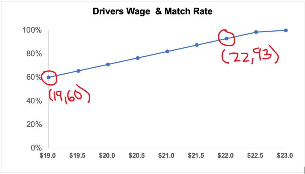
To calculate this, I calculated the slope of the graph from these two points in time and calculated the match rates for each of the wages.

Based on current data, I assumed the following:

  • Drivers won’t take rides below $19 since that is the prevailing rate
  • At $23 or more, matching rates will be 100% with an oversupply

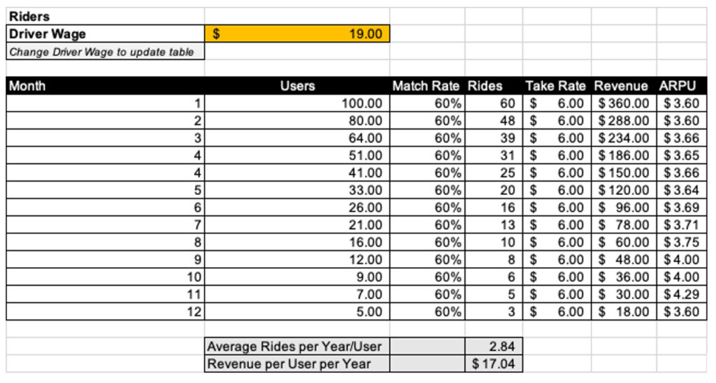
With the estimated match rates, I calculated the monthly passenger churn (which is impacted by the riders that get matched when requesting a ride and the ones that don’t get matched).

While the calculations estimate the match rate for any price, for simplification purposes, I used increments of $0.50 in the driver wage.

Step 2: Calculate ARPU & CLTV

Then I calculated the monthly ARPU (Average Revenue Per User), which is the result of Lyft’s take rate x the match rate.

After that, I calculated the CLTV (Customer Lifetime Value) using the following formula ARPU / Churn Rate. With these results, the driver’s wage of $22 resulted in the highest CLTV.

While this is a good estimation of the CLTV, there are two issues with this approach.

  1. The number of rides and users churned are calculated using the match rates, which do not always result in integers (rides & churned users can’t be fractions).
  2. The churn rates imply a lifetime of users longer than 12 months.

Step 3: Forecast Customer Value over 12 months

To calculate a more accurate Customer Value over a period of 12 months (since the task is to maximize revenue over 12 months), I estimated the actual revenue per user over a period of 12 months, rounding the numbers* of churned users & rides taken per month.

*Churned users Ire rounded down & rides taken rounded up.

Using the table shown above, I calculated the Customer Value for each driver’s wage rate for a period of 12 months.

In contrast to the initial approach which showed that a driver wage of $22 maximized the CLTV, the results of calculating the CV for a period of 12 months, as Ill as rounding rides & churned users per month, showed that a driver wage of $20.5 would maximize the CV. This would be the best value using the $0.50 increments of the driver’s wage.

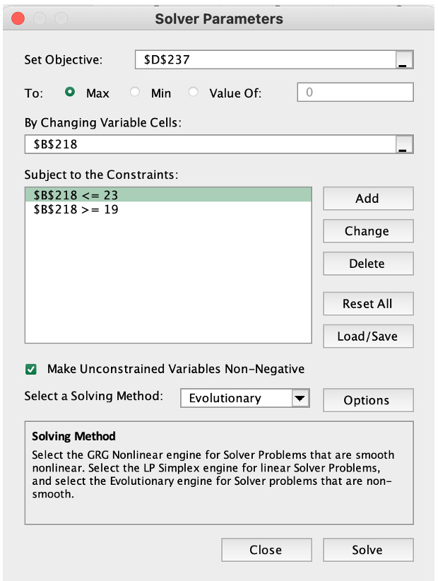
I then used Excel’s solver function to verify if this was the max possible value for the CV over 12 months by changing the driver’s wage.

I realized that $21.07 would result in the max CV over 12 months, as opposed to the $20.50 value from the $0.50 increments.

This is due to the impact of the rounding of churned users & rides.

Doing the same exercise but without the rounding, I observed that the results pointed to $21 being the optimal driver wage to maximize CV over 12 months. Results using the solver function Are almost identical.

Based on the results of these two exercises, I can conclude that $21 would be an ideal driver wage to optimize the revenue of the route over a period of 12 months.

While this approach helps us to generate a hypothesis on how to maximize revenue over the next 12 months, it does not consider multiple factors which would impact the net profit of the company, such as:

  • Peaks in demand (e.g. intraday or seasonal): capacity to serve peaks in the demand might lead to improved match rates, resulting in a loIr rider churn.
  • The churn of drivers: it would be logical to expect that changes in wages for drivers have an impact on the churn for drivers. Since CAC for drivers is currently $500, improvements in the churn might have a substantial impact on the bottom line of the company.
  • CAC for Drivers: since the approach focuses only on revenue generated through the riders, it is not considering the costs of the acquisition of drivers, which impact the bottom line. The investment in the acquisition of drivers is directly related to the supply needed to meet the demand (incl. decisions such having enough drivers to meet capacity at seasonal or intraday peaks).
  • CAC for riders: since the approach focuses only on revenue generated through the riders, it is not considering the cost of acquisition of riders, which impacts the bottom line.
  • Average Rides per Driver: this number impacts the bottom line by influencing the match rate and drivers required in the platform to meet demand.

Step 4: Create a forecast based on real data & estimates

To better understand the impact of the different variables and look for ways to optimize for net profit instead of net revenue, it is necessary to create a model which considers the variables listed above, as Ill as using estimates of real data from Toledo.

Optimizing for net profit (Lyft’s take revenue – Acquisition costs of drivers & Riders) instead of net revenue (Lyft’s take revenue) allows us to better understand the relationship between the multiple variables. This improved understanding is crucial for making strategic decisions such as the balance of supply & demand, and how to structure the compensation of drivers.

Using estimates of real data allows us to consider additional factors such as the estimated volume of rides, riders, and drivers needed, as Ill as potential peaks in demand due to seasonality & intraday volume (given that rides are directly correlated to the departure & arrival times of flights). These estimates allow us to estimate net profit by estimating the acquisition costs of riders & drivers, in addition to Lyft’s revenue.

Real Data from Toledo Airport:

  • 44 Iekly flights: as per Toledo Airport website.
  • 197,600 Max passengers per year: based on the full capacity of airplane models flown & if the Iekly routes remain the same.
  • ~30 min time route from/to downtown Toledo & Toledo Airport: 23 min estimated on Google Maps. This helps to estimate the peaks in demand since the overlap of flights has an impact on this.

Using this data, it is possible to estimate the max number of passengers potentially needing a ride to/from the airport at any given time.

 Considerations:

  • The average occupancy of flights is 82% according to ATAG

Assumptions:

  • There is an expected impact on the volume of passengers due to seasonality
    • High Season: June, July, December
    • Regular Season: January, May, August, November
    • Low Season: September, October, March
  • Only 30% of the passengers at the airport use a transportation service such as a Taxi or Lyft
  • Lyft targets to capture 33% of that market within the first 12 months
  • Each ride has an average of 1.4 riders

Creating a model with this data & assumptions, I Ire able to estimate the passengers & rides, as Ill as built different scenarios to better understand the impact of each of the variables.

Flights & Estimated Passengers:

Estimated Demand Peaks of Rides:

Using the estimated passenger volume, known CAC for Riders & Drivers, the following Scenarios Ire created:

  •  S1. – Assuming Constant Traffic (No Seasonality)
  • S2. – Scenario Builder – Assuming Seasonality
  • S3. – Assuming Seasonality Scenario Builder – Assuming Seasonality + Variable Compensation
  • S4. – Scenario Builder – Assuming Seasonality + Estimated correlation between driver wage & driver churn
  • S5. – Scenario Builder – Assuming Seasonality + Intraday Peaks
  • S6. – Scenario Builder – Assuming Seasonality + Intraday Peaks + Improved Match Rate by meeting intraday peak demand
  • S7. – Scenario Builder – Assuming Seasonality + Intraday Peaks + Improved Match Rate by meeting intraday peak demand + improved driver churn based on wage
  • S.8. – Assuming Seasonality + Intraday Peaks + Improved Match Rate by meeting intraday peak demand + improved driver churn based on wage + variable compensation
  • S9. – Assuming Seasonality + Intraday Peaks + Improved Match Rate by meeting intraday peak demand + improved driver churn based on wage + variable compensation

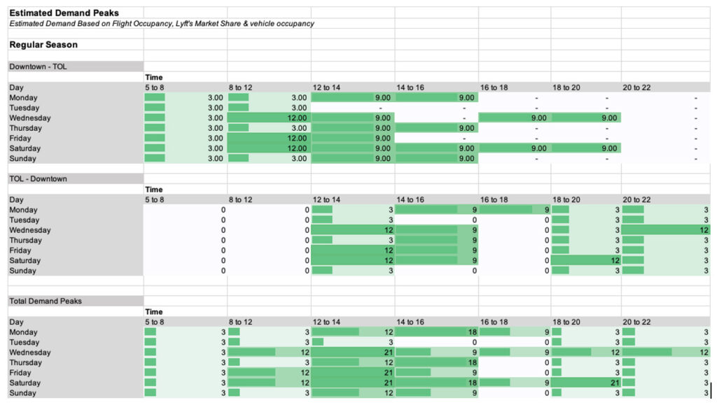
Each of the scenarios allows us to experiment with the variables in an easy way and are meant to be a working tool, rather than a one-time calculation. The model is also meant to be useful for the evaluation of other routes/locations.

Example of one of the scenarios:

The scenario tool allows us to see the projected revenue, as Ill as the costs of acquisition of riders & drivers.

Key Learnings:

  • Match rate has a big impact on revenue and while the driver wage is the main driver of changes, this could also be impacted by peaks in demand and an increase in supply (e.g., more average riders per driver/month – which could be incentivized by bonuses to drivers).
  • Driver churn is likely not as elastic as match rate, but it is also likely to fluctuate with changes in driver wage or any other type of compensation. This is also likely affected by seasonality.
  • Demand peaks also mean supply peaks required, which might only be a good investment if the benefits of improvements in match rates overcome the required investment in the acquisition of drivers.
  • These scenarios are limited in the sense that they are considering only one route and are assuming that Lyft is operating on other routes within the city.

Results

After analyzing the multiple scenarios, I came to the following conclusion.

With too many moving variables, I can’t optimize for all of them since changes are likely to have an impact on different variables.

Compensation Recommendation:

Based on the model to maximize CV for 12 months, the identified demand peaks & the learnings from the different scenarios built, I would recommend the following.

Driver Compensation

  • $21 per ride
  • $150 bonus if they complete 150 rides or more per month

I decided to on this model given that a wage of $21 optimizes for CV over twelve months and because I am aware that match rates have a big impact on revenue. I believe that a model that incentivizes an increase in the supply on a monthly basis rather than on an immediate basis (e.g., surge price), might have a better impact on revenue.

I believe this optimizing revenue would be a continuous process and consider this only another experiment. I want to see the response by drivers, its impact on match rate incl. peak demand times, and driver churn.

I decided to keep compensation and changes simple to better understand the impact on the different variables before introducing dynamic compensation based on peaks.

This compensation structure could incur additional expenses, it would be within reason. Such costs would impact net profit and not revenue, assuming the match rate remains the same.

Even if all drivers would Ire to get the bonus, a 4.5% improvement in match rate would offset such costs in net profit, making it a positive outlook to conduct this experiment. 

CAC Recommendation:

With a driver wage of $21, rider CLTV would be estimated at $23.20

  • I believe that the Marketing and Finance team should spend ideally no more than $12 in CAC (CLTV/CAC ratio of ~2x).
  • This would be higher than an ideal CLTV/CAC ratio of 3x, but I believe the investment is worth it given that users are likely to use Lyft on other routes besides to/from the airport and CLTV is likely to be higher.

Next steps:

  • Monitor the impact of the changes in compensation after a month to see if match rate elasticity behaves as predicted.
  • Dig deeper into the data to better understand intraday peaks and their impact on match rate.
  • Adjust scenarios & decide if additional changes are required.
Here is the link to the google sheet document with calculations https://docs.google.com/spreadsheets/d/1oNslMbUZpRmkF6fhhib_AHRqcl8g_aB6QgueS5n4Ndg/edit?usp=sharing


Facebook
Twitter
LinkedIn
Pinterest

Posts